THAT: THe Analog Thing
Disclaimer: I am not affiliated with anabrid GmbH and this post is not sponsonsored by them or anyone else. I have purchased The Analog Thing myself, and I do not gain anything if you decide to purchase one for yourself after reading this post.
Introduction
THe Analog Thing (also called THAT) is a “low-cost, open-source, and not-for-profit” general purpose analog computer which can be purchased today as new. I say “today and as new” on purpose, because analog computers are (or were?) part of history. They had their golden age ~60 years ago.
This post is very brief, for a detailed information from an expert, I highly recommend the book Analog Computing by Prof. Dr. Bernd Ulmann, who is also one of the founders of anabrid GmbH, the company behind THAT. I also recommend his other book, Analog and Hybrid Computer Programming.
I plan to update this post as I learn more while spending more time with my THAT(s).
Why Analog is not only not-Digital
When one hears the term “analog computer”, the first thing that comes to mind is this is a computer that is built from “analog electronic circuits” as opposed to “digital”, thus using continuous voltages, as opposed to zeroes and ones of digital computers. However, this is not the whole story and it is not the important part of the story.
The issue is I think caused by two somehow related meanings of the word “analog”. However, one of these meanings became too strongly associated with what we think when we hear “analog” in electronics. Oxford Languages Dictionary gives the two following meanings for the word “analog”:
“relating to or using signals or information represented by a continuously variable physical quantity such as spatial position, voltage, etc.”
“a person or thing seen as comparable to another.”
Probably the reason analog electronics is called “analog” is because there is a “proportional” relationship between the signal and the voltage or the current (whereas in digital electronics there is an encoding, not a proportional relationship). This comes from the (ancient) Greek word ανάλογος (analogos) which also means “proportionate” or “proportional”.
On the other hand, Oxford Languages Dictionary defines “digital” as:
“(of signals or data) expressed as series of the digits 0 and 1, typically represented by values of a physical quantity such as voltage or magnetic polarization.”
“(of a clock or watch) showing the time by means of displayed digits rather than hands or a pointer.”
“relating to a finger or fingers.”
(if we go further, it seems the Latin word comes from Proto-Italic and Proto-Indo-European words meaning to show or point out, since one points with fingers)
I did not realize “digital” comes from the Latin word “digitus” which means finger or toe. I guess because one can count with fingers, and a count is represented with numbers, digit started to have the current meaning.
Since in digital electronics, countable number of states are used, the use of digital here also makes sense.
However, digital is started to give the sense of opposite of analog. Thus, digital corresponds to countable and binary, whereas analog corresponds to uncountable and/or continuous. This is naturally true to some extent, however, it misses a very important point. The important point is the second meaning of “analog” given before; “a person or thing seen as comparable to another”. To elaborate this, I should say a few things about the levels of abstraction.
Assume we have a problem. For the sake of this article, it is much easier to think of a problem that can be described by differential equations.
A digital computer program to solve this problem would be an implementation of a numerical analysis method (such as Runga-Kutta method). Another (similar or different) problem would also be solved with a (similar or different) program but running in the same computer architecture. The hardware architecture does not change for the problem, but the programs change.
On the other hand, a solution to this problem on an analog computer would be to wire the patch cables correctly to create an “analog” of the problem on the analog computer. Here, the analog of the problem is created with a structural analog on an electronic hardware. Thus, in this configuration, the analog computer works only for this problem. Another problem requires another physical configuration. Thus, not the program (or program memory, there is no such memory in an analog computer), but the physical configuration also changes as the problems change. Moreover, the analog computer itself, when runs, does not only solve the problem but actually behaves like the problem. The analog computer is more close, less abstract, than the digital computer to the problem. This is the difference that is missed when only analog voltages are understood with the term analog computer. Because of this, I think, in many cases, it makes more sense to say that an analog computer is simulating the equations rather than solving the equations.
The integrator below does not calculate an integration but it is inherently the integration itself.
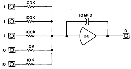
Integrator Simplified Schematic (ref: TR-48 Analog Computer Operators Manual)
Another nice way to phrase this, which I heard in a talk by Prof. Ulmann, is that the memory in a digital computer isolates the computer hardware from the problem. If the problem (the program that describes the solution of a problem) fits to the memory of a digital computer, then it can be solved. On an analog computer, there is no memory. Thus, the analog computer hardware has to match with the problem. If the problem matches or fits to the analog computer hardware, then it can be solved. That is why there is a hard-limit in analog computing, if a problem requires more computational elements, then it cannot be solved. This difference, memory requirement vs. hardware requirement, reveals itself also in the solution time. A digital computer runs the program, and this execution speed determines the solution time of the problem. On an analog computer, within the limitations of electronic circuits, there is no such limitation, the execution speed is basically determined by the time constant of integrators, basically depending on the passive elements, capacitors and resistors.
I think, theoretically, if the problem is both discrete in time and in state space, this problem can also be solved by a “digital computer” like an “analog computer” in the sense the digital computer can be made general purpose and patched to be an analog of the problem.
I should add there is another category here which looks like an “analog computer” but it is not a general purpose computer and it has less (maybe no) abstraction. It is naturally possible to build an electronic (analog or digital) circuit that directly represents either the system or it is the system itself (such as Chua’s circuit). This type of direct computation or representation is not a general purpose analog computer. It works similar to an analog computer, however, because it has less or no abstraction, it can be much more compact. For example, Chua’s circuit is much more compact than simulating it on an analog computer, because any components can be used and the circuit can be freely designed.
a Chua's Circuit prototype I made
Electronic analog computers
History
For centuries, and particularly in last 300 years, analog computers are implemented with mechnical components. One of the latest use of such a mechanical computer was for example the Norden bombsight which was also used in the bomber plane Enola Gay which dropped the atomic bomb on Hiroshima on 6 August 1945.
In 1930s and 1940s, it is realized that an analog computer can also be implemented electronically, using electronic components instead of mechanical components. An important result of this was the decision to use integrators instead of derivators (both operations can be electronically implemented similarly). The reason is that integration functions like a low-pass filter, and filters out the generated noise, whereas the noise increases with derivation. When I say analog computer from this point on, I mean electronic analog computer in this post.
In late 1940s, 1950s and 1960s, there was a lot of development, interest and use. I think in late 1960s and then 1970s, because certain issues are addressed better with a digital computer, analog hybrid computers were developed. These are as you expect a combination of analog computer and a digital computer, either running sequentially (one after another or alternating) or running together. During 1970s, due to major developments in digital computers, and their certain advantages over analog computers, analog computers became unpopular and replaced by digital computers. The last analog computers were in use in 1980s.
Lately, there is an increasing interest in analog computing architectures (not only electronic but also biological), where a major reason is energy efficiency.
Operational amplifier (OPAMP)
Operational amplifier (OPAMP) is a basic active electronic component. It is much more complicated than a single transistor (see the functional block diagram below) but it can be used as a basic component because it has a very basic function. It is not straightforward now to see why it is called “operational”, but actually the name comes from the fact that these are first used for mathematical operations in analog computers. The development of OPAMP was critical for analog computers and after eliminating the drift (by invention of chopper stabilization), they become the computational unit of the analog computers. Since they are used for all basic operations (integration, sum), an analog computer always mention how many amplifiers (meaning OPAMP) it contains.
THAT uses TI’s TL074H operational amplifier.
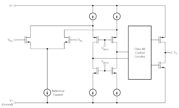
TI TL074H functional block diagram (ref: ti.com)
Using an analog computer
Before an analog computer is used, a mathematical model of the problem is created, this is basically a set of differential equations. This is probably done by someone else other than the analog computer user or together with an expert, because it might require an expertise in a particular domain. Also, not all problems fit well to analog computers.
When the mathematical model/differential equations are available, the basic steps of using an analog computer is like this:
- The differential equations are reorganized to be implemented as integrators. (e.g. by using Kelvin’s feedback technique or Substitution method)
- The variables and constants are scaled to fit to the operating range of the analog computer. Because analog computer operates at a fixed voltage range, any variables at any time should stay in this range, if not, the result would be invalid.
- The equations are mapped to the analog computer by using the patch panel by connecting various points in the analog computers with patch cables.
- The parameters, including initial values, are set using the potentiometers on the analog computer.
- The analog computer is run.
- The outputs are observed on voltmeter or oscilloscope or saved by a plotter or multi-channel recorder.
Overload
Preventing overload is a must for analog computers, and it should be addressed at the beginning, before creating a patch. On a digital computer, using floating-point numbers, there is usually no problem of overloading. Even when using integer numbers, the problem is easier to resolve. For analog computing, preventing overload means magnitude scaling. This means replacing the variables in the original equation with scaled ones.
Precision and measurement
The precision in analog computing is, I think, theoretically infinite since it works on continuous values but practically it is very limited due to noise in the system. The physical nature of the classical analog computer also limits the options to minimize the noise. Thus, the precision in analog computing is usually $10^{-4}$ at best. This is approx. 14-bits in a digital system ($2^{14} = 16384$).
As opposed to digital computers, the result of analog computation must be explicitly measured since the results are not stored in memory or registers. An analog computer outputs a voltage proportional to a (scaled) variable in the problem. This voltage is measured and then displayed, plotted or printed. Thus, the measurement also affect the overall precision, and the measurement device should have a similar or better precision than the analog computer. For a digital measurement system, this means the analog computer output should be measured with 12-16 bit resolution. For 14-bit, it means a 5.5 digits voltage measurement. The measurement is problematic with old/cheap or fast digital oscilloscopes, they usually have 8 or 10 bit resolution.
Interactivity and programmability
Because the time scale of analog computation and the operating time can be adjusted easily, it can be run repeatedly. Since the (analog) simulation is running in real-time, response to controls (adjustments of coefficients or changes in other inputs) are immediate. When the digital computation can be done quickly, it can behave similarly but it is not a property of the system as in the analog simulation.
When you know what to do (i.e. you know the problem and you have mapped and scaled the problem to the analog computer), “programming” -patching might be a better term- an analog computer is much simpler as there is only a light physical interaction (e.g. plugging some cables, turning some knobs) needed. Even a small child can easily make a patch on an analog computer and run it. This is much more complicated with digital computers. Using an analog computer is much simpler and naturally more direct, even when compared to child friendly programming environments in digital computers.
Interactivity and programmability of an analog computer makes it a powerful tool for teaching and studying the dynamical systems and the natural phenomena described by a dynamical system.
Electronic Associates, Inc. (EAI) TR-20
I do not know the market share of companies which were producing analog computers. However, probably the most famous company in this area was Electronic Assoicates, Inc. (EAI), which was founded in 1945 and started making analog computers in 1952.
One of their product was PACE TR-20, launched in 1963. This was a table-top computer, for education or for basic research. It was also solid-state (transistor based, not vacuum tube). I think its features are similar to THAT, that is why I mention this model. Be aware that it is one of the most basic models, there are a lot larger analog computers than TR-20. It has a larger sibling, called TR-48.

PACE/EAI TR-20 (ref: wikichip.org)
Because the components of TR-20 are solid-state, its operating voltage is +-10V (not +-100V as with vacuum tube based computers). This is also true for THAT.
TR-20 has -not surprisingly- 20 amplifiers (opamps). It is possible to use each amplifier as a summer, integrator or an open loop (high-gain) amplifier. TR-48 has 48 amplifiers.
In addition to amplifiers, it has a selection of different components such as quarter-square multiplier (for multiplication and division), X^2 diode-function generator, log function, comparator. It has two time scales, real-time and HSRO (500x times faster). Its resistor networks are matched to have 0.01% accuracy.
The Analog Thing (THAT)
As mentioned before, THAT is aimed to be a low-cost (and not-for-profit) analog computer. To do that, every possible decision seems to be made in order to decrease its cost. However, this does not mean it has a low quality. I am using it for only a few weeks, so I cannot say something about reliability, but the overall build quality is very good. At the moment, it costs 419 Euros (378 with academic discount).
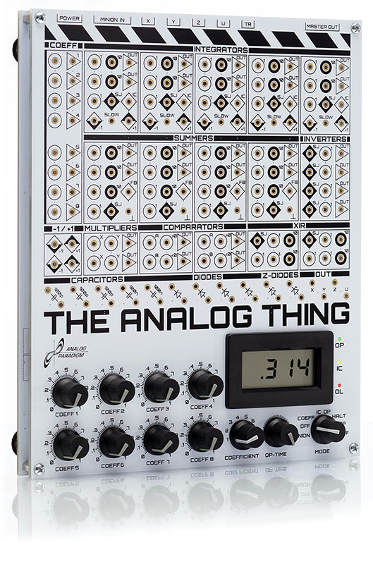
The Analog Thing (ref: the-analog-thing.org)
It has a very similar size to an A4 page, on the long edge shorter than the A4 page.
It does not have a case, and basically consists of two PCBs. The bottom/base PCB is the main board, where all the important circuitry stays. The top/front PCB is where all the connectors are and also functions as a front panel. Because connectors are expensive, and there are many connectors on an analog computer (THAT has almost 200), it very cleverly avoids using connectors and uses gold plated holes on the PCB. In order to improve connectivity, there is a plastic material under the front panel and small banana jacks (2mm) can half enter into the plated holes.
Being an open hardware, the schematic and gerber files of THAT is available on github.
It is also possible to chain more than one THATs very easily, where one functions as master and all of them runs together, effectively increasing the number of computing elements.
If you buy a THAT, I highly recommend to buy an extra package of patch cables. You might need it or keep as backup. I am not sure how easy to find 2mm banana patch cables, to my knowledge they are not very common.
I could find only three things that I would change on THAT.
The number of computing elements are pretty good but it would be nice to have more than 2 multipliers. The multiplier IC is an important cost, I think that is the reason for having only two multipliers. Keep in mind that THATs can be connected and work together, so any limitation in computing elements can be overcome by using multiple THATs. I demonstrate this in the Chua oscillator demo at the end of the post.
The coefficient potentiometers are single turn, so they are not very precise. I am not 100% sure how important this is, but it would be nice to have 3 turn potentiometers, maybe not for all but only for a few of them.
Not sure the current rating of the internal 5V to 12V,-12V power regulator, but I wish it had an easy to access (terminal block etc.) to 12V, -12V and GND for custom expansions.
Overall, I think THAT is great. If you know a high-school/university student who is interested in dynamical systems, it would be a great gift. I think it is a great teaching tool for schools, even if it is used just for one demo in one lab or lecture hour, it would inspire some students.
Output and Display
THAT has five outputs on the back provided with RCA/cinch connectors. Four of the outputs are X,Y,Z,U that would normally be related to computation. The last output is TR, trigger output, which is a 5V active-low signal. When THAT is operating, TR is low (0V), otherwise it is high (5V).
It is important to understand that THAT on its own is not enough to make a reasonable analog computation exercise. An analog computer like THAT usually only comes with a voltmeter on board, and it has outputs to be connected to a more advanced display/output unit such as a scope (oscilloscope), plotter, multi channel recorder etc. The scope and plotter might have XT (time on horizontal axis) and/or XY modes. For THAT, it means you need an oscilloscope.
Unfortunately, for someone who does not have any other test instruments but want to try THAT, I think this can be the most problematic point as something else has to be purchased. There are some oscilloscope options listed on the wiki of THAT and also some other (cheaper) options such as sound cards. I cannot comment on any of these since I dont use any but I can tell what I think would be good to have in an output device:
more than 2 channels, this usually means 4. It is not a must, but if you want to see 3 variables, it is not a nice limitation to have, and there are many third-order dynamical systems, particularly the chaotic systems.
capability to display XT and XY, both at the same time, and various combinations of these. The more flexible the device is in this regard, the nicer the experience will be, particularly for third or more order dynamical systems.
a separate trigger input is good to have, otherwise you should be able to use one input as trigger (but this will consume one channel). It might be OK to use an existing channel (x,y,z) as trigger but it is again nicer and convenient to use the trigger output on THAT for this purpose.
PicoScope
I have a better PicoScope (4424A) than the one on the wiki of THAT (which mentions PicoScope 2000 series). I already had this scope and it has all the things I said above except the separate trigger input (and I use one channel as trigger), so it is quite nice to use it with THAT. However, the new price of this scope is as much as three THATs, so it does not make sense to recommend it only for THAT. It has 4 channels and display capability is very good.
National Instruments DAQ
Another option might be to use a National Instruments data acquisition (DAQ) system. If you are not familiar with NI’s products, they are expensive and cover a very wide range. There are simple devices (like a small USB box), and very advanced ones. The good thing is you can use LabVIEW to program the DAQ device to acquire and visualize the signals as you like. When purchased new, they are (much) more expensive than THAT, but you may find a reasonably priced used one. Also, LabVIEW offers a free community edition for non-commercial use. I have a few NI products, and using USB-6351, I made a “virtual instrument” in LabVIEW, called THATscope, which shows many things including a 3D view and adjust the shown time range to trigger pulse width.
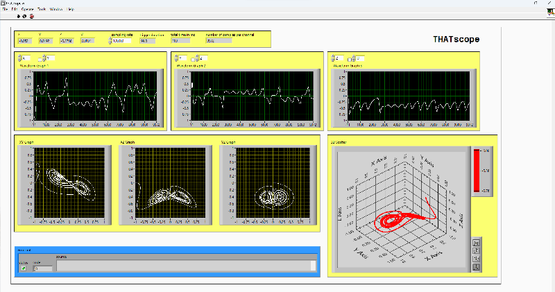
THATscope showing Lorenz (Butterfly) Chaotic Attractor
Other than its price, I think the main problem with these devices is that it is hard to find one that fits well to this purpose. Most of the “normal” devices with analog input samples maximum around 1MS/s (like USB-6351), and this is not simultaneous, so using 4 channels, this means 200kS/s or so. However, it offers more resolution than needed, USB-6351 has a 16-bit ADC. You might find one with more than 1MS/s and simultaneous sampling, but then it will be expensive. Other option is to use a high speed digitizer or oscilloscope system, but again this will be expensive. I do not see a device similar to PicoScope, more than 10MS/s but at 12-bit. I think it is possible to use PicoScope with LabVIEW, I have not tried it yet.
Demos
I think reading about analog computers does not give an enough feeling of how they work. So I recorded two videos showing two examples.
First is probably one of the most simple examples, radioactive decay. It is described both in the manual of THAT, and in the book Analog and Hybrid Computer Programming.
Second is an important one but it is not given in the manual, van der Pol oscillator. It is described also in the book Analog and Hybrid Computer Programming.
Radioactive decay
A radioactive material contains unstable atomic nuclei. An unstable atomic nucleus decays into a stable form. There are various mechanisms behind this, like emitting $\alpha$ particles, and it is not possible to predict when a particular atom will decay. However, on a macro scale, the overall decay rate is constant, and expressed as a decay constant or as half-life.
Using the decay constant, which is denoted by $\lambda$:
$A = -\dfrac{N}{t} = \lambda N$
where:
- $A$ denotes the activity, or the number of decays per unit time
- $N$ denotes the number of particles (atoms etc.) in the sample
The initial number of particles is $N_0$.
Radioactive decay is described with this first-order differential equation:
$\dot{N} = - \lambda N$
which can be easily mapped into the analog computer:
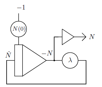
Computer setup of radiactive decay problem (ref: Figure 4.3 in Analog and Hybrid Computer Programming)
After patching this setup on THAT, I have taken the video below, where I start by setting up the coefficients for the initial condition ($N_0$ and $\lambda$), then start the operation and modify the coefficients while running.
van der Pol oscillator
Prof. van der Pol received his Ph.D. in 1920 and joined Philips Research Laboratories in Netherlands. He invented the term and the concept of “relaxation oscillations” and his studies on what we call now “van der Pol equation” is an important milestone in nonlinear dynamical systems theory.
Relaxation oscillation means the system stores energy and periodically releases the stored energy, hence it is an oscillation. There are many natural analogs of this phenomena such as heartbeat, action potential (of neurons) and earthquakes. The first paper Prof. van der Pol published about this topic was a model of heart.
van der Pol oscillator is described with a second-order differential equation:
$\ddot{y} + \mu(y^2 - 1)\dot{y} + y = 0$
This problem is not as easy as the radioactive decay to map into the analog computer. Here, I use the approach described in the book (Analog and Hybrid Computer Programming) which results in this setup:
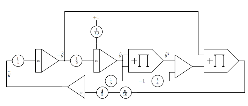
Computer setup of van der Pol oscillator (ref: Figure 6.16 in Analog and Hybrid Computer Programming)
Like with radioactive decay, after patching this setup on THAT, I have taken the video below. In this video, there are two scope views, the second one is an XY view to observe the limit cycle. As you can see the OL (overload) indicator is on, and it is because one of the integrators are just touching its maximum. I am not sure why the equation is scaled like this in the book, maybe it works fine with Analog Paradigm Model-1.
Lorenz attractor
This is probably the most famous chaotic system shown by Edward Lorenz in 1960s. It displays the chaotic attractor, also called butterfly attractor which gave its name to butterfly effect.
It is described by the following third-order system given in three first-order equations:
$\dot{x} = \sigma (y - x)$
$\dot{y} = x (\rho - z) - y$
$\dot{z} = xy - \beta z$
The patch is naturally more complex than van der Pol oscillator.
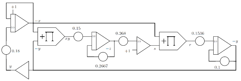
Computer setup of Lorenz attractor (ref: Figure 6.45 in Analog and Hybrid Computer Programming)
I patched it as described in the manual of THAT, and here is a short video:
Chua oscillator
This is another famous chaotic system described by Chua in 1980s. It can display a lot of different behavior and below the double scroll attractor is shown.
It is described by the following system:
$\dot{x} = c_1 (y - x - f(x))$
$\dot{y} = c_2 (x - y + z)$
$\dot{z} = -c_3 y$
where
$f(x) = m_1 x + \frac{m_0 - m_1}{2} (|x+1| - |x-1|)$
The patch implementing this system is quite complex because it requires absolute value to implement the piece-wise linear function $f(x)$. A single THAT is not enough, even two THATs are barely enough. I used all summers, inverters and XIRs of two THATs.
The patch is described in the book, Analog and Hybrid Computer Programming, however there is a typo in the book, one of the attenuator values are shown wrong (in Figure 6.52). The same patch is described also in the application note 3 with the correct values.
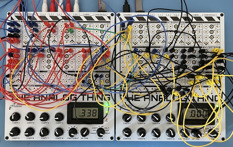
Using two THATs for Chua oscillator
I am also using my LabVIEW virtual instrument to visualize this patch:
This work is licensed under a Creative Commons Attribution-NonCommercial-ShareAlike 4.0 International License.